
Hadoop Analytics 101
Apache Hadoop by itself does not do analytics. But it provides a platform and data structure upon which one can build analytics models. In order to do that one needs to understand MapReduce functions so they can create and put the input data into the format needed by the analytics algorithms. So we explain that here as well as explore some analytics functions.
Hadoop was the first and most popular big database. Products that came later, hoping to leverage the success of Hadoop, made their products work with that. That includes Spark, Hadoop, Hbase, Flink, and Cassandra. However Spark is really seen as a Hadoop replacement. It has what Hadoop does not, which is a native machine learning library, Spark ML. Plus it operates much faster than Hadoop since it is an in-memory database.
Regarding analytics packages that work natively with Hadoop – those are limited to Frink and Mahout. Mahout is on the way out so you should not use that. So your best options are to use Flink either with Hadoop or Flink tables or use Spark ML (machine language) library with data stored in Hadoop or elsewhere and then store the results either in Spark or Hadoop.
(This article is part of our Hadoop Guide. Use the right-hand menu to navigate.)
Analytics defined
In order to understand analytics you need to understand basic descriptive statistics (which we explain below) as well as linear algebra, matrices, vectors, and polynomials, which you learn in college, at least those who pursued science degrees. Without any understanding of that you will never understand what a K-Means classification model or even linear regression means. This is one reason regular programmers cannot always do data science. Analytics is data science.
Analytics is the application of mathematical, statistics, and artificial intelligence to big data. Artificial intelligence is also called machine learning. These are mathematical functions. It is important to understand the logical reasoning behind each algorithm so you can correctly interpret the results. Otherwise you could draw incorrect conclusions,
Analytics requires a distributed scalable architecture because it uses matrices and linear algebra. The multiplication of even two large matrices can consume all the memory on a single machine. So the task to do that has to be divided into smaller tasks.
A matrix is a structure like:
[a11, a12, a13,...,a1n
A21, a22, a23, … a2n
…
A i1, ai2, ai3, …, ain]
These matrices are coefficients to a formula the analyst hopes will solve some business or science problem. For example, the optimal price for their product p might be p = ax + by + c, where x and y are some inputs to manufacturing and sales and c is a constant.
But that is a small example. The set of variables the analyst has to work with is usually much larger. Plus the analyst often has to solve multiple equations like this at the same time. This is why we use matrices.
Matrices are fed in ML algorithms using Scala, Python, R, Java, Python, and other programming languages. These objects can be anything. For example, you can mix and match structures:
Tuple(a,b,a)
Tuple(int, float, complex number, class Object)
Array (“employees:” “Fred”, “Joe”, “John”, “William)
So to use Hadoop to do analytics you have to know how to convert data in Hadoop to different data structures. That means you need to understand MapReduce.
MapReduce
MapReduce is divided into 2 steps: map and reduce. (Some say combine is a third step, but it is really part of the reduce step.)
You do not always need to do both map and reduce, especially when you just want to convert one set of input data to a format that will fit into a ML algorithm. Map runs over the values you feed into it and returns the same number of values that you fed into it but changing that to a new output format. The reduce operation is designed to return one value. That is sort of a simplification, but for the most part true. (Reduce can return more than one output. For example, it does that in the sample program we have shown below.)
MapReduce example program
Here is the Word Count program copied directly from the Apache Hadoop website. Below we show how to run it and explain what each section means.
First you need a create a text file and copy it to Hadoop. Below shows its contents:
hadoop fs -cat /analytics/input.txt
Hello World Bye World
The program will take each word in that line and then create these key->value maps:
(Hello, 1)
(World, 1)
(Bye, 1)
(World, 1)
And then reduce them by summing each value after grouping them by key to produce these key->value maps:
(Hello, 1)
(World, 2)
(Bye, 1)
Here is the Java code.
package com.bmc.hadoop.tutorials;
import java.io.IOException;
import java.util.StringTokenizer;
import org.apache.hadoop.conf.Configuration;
import org.apache.hadoop.fs.Path;
import org.apache.hadoop.io.IntWritable;
import org.apache.hadoop.io.Text;
import org.apache.hadoop.mapreduce.Job;
import org.apache.hadoop.mapreduce.Mapper;
import org.apache.hadoop.mapreduce.Reducer;
import org.apache.hadoop.mapreduce.lib.input.FileInputFormat;
import org.apache.hadoop.mapreduce.lib.output.FileOutputFormat;
public class WordCount {
public static class TokenizerMapper
extends Mapper<object , Text, Text, IntWritable>{
private final static IntWritable one = new IntWritable(1);
// Text is an ordinary text field, except it is serializable by Hadoop.
private Text word = new Text();
// Hadoop calls the map operation for each line in the input file. This file only has 1 line, // but it splits the words using the StringTokenizer as a first step to createing key->value // pairs.
public void map(Object key, Text value, Context context
) throws IOException, InterruptedException {
StringTokenizer itr = new StringTokenizer(value.toString());
while (itr.hasMoreTokens()) {
word.set(itr.nextToken());
// This it writes the output as the key->value map (word, 1).
context.write(word, one);
}
}
}
// This reduction code is copied directly from the Hadoop source code. It is copied here // so you can read it here. This reduce writes its output as the key->value pair (key, result)
public static class IntSumReducer
extends Reducer {
private IntWritable result = new IntWritable();
public void reduce(Text key, Iterable values,
Context context
) throws IOException, InterruptedException {
int sum = 0;
for (IntWritable val : values) {
sum += val.get();
}
result.set(sum);
context.write(key, result);
}
}
public static void main(String[] args) throws Exception {
Configuration conf = new Configuration();
Job job = Job.getInstance(conf, "word count");
job.setJarByClass(WordCount.class);
// Here we tell what class to use for mapping, combining, and reduce functions.
job.setMapperClass(TokenizerMapper.class);
job.setCombinerClass(IntSumReducer.class);
job.setReducerClass(IntSumReducer.class);
job.setOutputKeyClass(Text.class);
job.setOutputValueClass(IntWritable.class);
FileInputFormat.addInputPath(job, new Path(args[0]));
FileOutputFormat.setOutputPath(job, new Path(args[1]));
System.exit(job.waitForCompletion(true) ? 0 : 1);
}
}
To run this you need to create the /analytics folder in Hadoop first:
hadoop fs -mkdir /analytics
Run the code like this:
yarn jar /tmp/WordCount.jar com.bmc.hadoop.tutorials.WordCount /analytics/input.txt /analytics/out.txt
Then check the output. First use hadoop fs -ls /analytics/out.txt to get the file name as the results are saved in the output.txt folder
hadoop fs -cat /analytics/out.txt/part-r-00000
Here is the resulting count.
Bye	1
Hello	1
World	2
Descriptive statistics
In order to understand these models analytics it is necessary to understand descriptive statistics. This is the average , mean (μ), variance(σ2), and standard deviation (□) taught in college or highschool. In statistics, the normal distribution is used to calculate the probability of an event. The taller the curve and the closer the points are together the smaller the variance and thus the standard deviation.
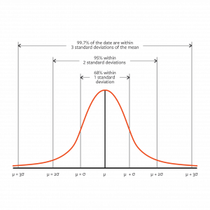
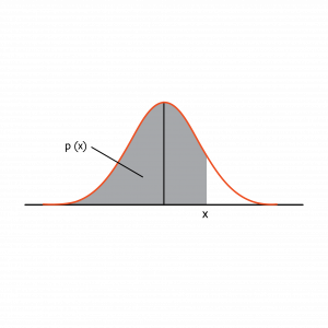
The normal curve is a graphical presentation of probability: p(x). For example, the probability that a value is less than or equal to x above is p(x).
Linear regression
Now we talk in general how some of the analytics algorithms work.
Linear regression is a predictive model. In terms of machine learning it is the simplest. Learning it first is a good idea, because its basic format and linear relationship remains the same for more complicated ML algorithms.
In its simplest form, linear regression has one independent variables x and 1 dependant variable y=mx +b.
We can graph that like this:
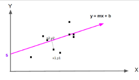
The line y = mx +b is the one such that the distance from the data points to the purple line is the shortest.
The algorithm for calculating the line in Apache Spark is:
org.apache.spark.ml.regression.LinearRegression
Logistic regression
In a linear regression we look at a line that most nearly fits the data points. For logistic regression we turn that into a probability. This outcome of logistic regression logit is one of two values (0, 1). This is associated with a probability function p(x). By convention when p(x) > 0.5 then logit(p(x))=1 and 0 otherwise.
The logistic regression is the cumulative distribution function shown below where e is the constant e and s is scale parameters.
1 / (1 + e**-((x -□) /s))
If that looks strange do not worry as further down we will see the familiar linear functions we have been using.
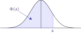
To understand that logistic regression represents the cumulative distribution under the normal curve, consider the point where x =□ in the normal curve. At that point x – □ = 0 so 1 / (1 + e**-((x – □) /s))=1 / (1 + e**((1 – 1 )/s)) = 1/ ( 1 + e**0) = 1/ ( 1 +1) = 1/2 = 0.5. That is the shaded area to the left of the y axis where x = □ In other words there is a 50% chance of a value being less that than the mean.The graph showing that is shown here again:
The logistic regression algorithm requires a LabeledPoint structure in Spark ML.
(labels, points)
Which we plugged into the LogisticRegressionWithLBFGS algorithm. The labels must be 1 or 0. The points (features) can be a collection of any values like shown below.
(1: {2,3,4})
(0:{4,5,6})
The data we feed in is called the training set. In other words it is a sampling of actual data. These are taken from past history. This lets the computer find the equation that best fits the data. Then it can make predictions. So if:
model = LogisticRegressionWithLBFGS (LabeldPoint of values)
Then we can use the predict function to calculate the likelihood, which is 1 or 0:
model.predict(1,2,3) = 1 or 0.
Odds
Logistic regression is difficult to understand but easier to understand if you look at it in terms of odds. People who bet on horse races and football certainly understand that.
odds =(probability of successes / probability of failure)
If you roll a dice the odds are (1/7)/(6/7) = ⅙. In logistic regression the outcome is either 0 of 1.So the odds are:
odds (y) = p(y=1)/ p(y=0) = p(y=1)/ (1 - p(y=1))
Logistic regression is the logarithm of the odds.Remember that the probability comes from some linear function like:
Odds (x) = a1x1 + b1x2 + c1x3 + d
The logarithm of that is :
log(Odds (x)) = log(a1x1 + b1x2 + c1x3 + d)
We undo that by raising by sides to e giving the original odds formula:
odds(x) = e**(a1x1 + b1x2 + c1x3 + d)
If that is difficult to see then consider the situation of a heart disease patient. We have a linear formula obtained derived from years of studying those. We can say that the chance of getting heart disease is some functions of:
(a1 * cholesterol) + (b1 * smoking) + ( c1 + genetic factors) + constant
That is a linear equation.
Support vector machines
With Support Vector Machine (SVM) we are interested in assigning a set of data points to one of two possible outcomes: -1 or 1. (If you are thinking that’s the same as logistic regression you would be just about correct. But there are some nuanced differences.)
How is this useful? One example is classifying cancer into two different types based upon its characteristics. Another is handwriting recognition or textual sentiment analysis, meaning asking whether, for example, a customer comment is positive or negative.
Of course a SVM would not be too useful if we could only pick between two outcomes a or b. But we can expand it to classify data between n possible outcomes by using pairwise comparisons.
To illustrate, if we have the possible outcomes a, b, c, and d we can check for each of these four values in three steps. First we look pair wise at (a,b) then (a,c) then (a,d) and so forth. Or we can look at one versus all as in (a, (b,c,d)), (b, (a,c,d)) etc.
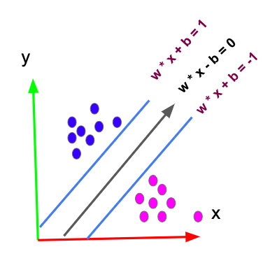
As with logistic and linear regression and even neural networks the basic approach is to find the weights (w) and bias (b) that make these formulae correct mx + b = 1 and mx + b = -1 for the training set x. m and x are vectors and m * x is the dot product m • x.
For example, if m is (m1,m2,m3,m4,m5) and x is (x1,x2,x3,x4,x5) then m •x + b is (m1x1 + m2x2 + m3x3 + m4x4 + m5x5) + b.
For linear regression we used the least squared error approach. We SVM we do something similar. We find something called a hyperplane. This threads the needle and finds a plane or line that separates all the data points such that all the weights and input variables are on one side of the hyperplane or the other. That classifies data into one category or the other.
In two-dimensional space the picture looks like shown below. The line m • x + b = 0 is the hyperplane. It is placed at the maximum distance between m • x + b = 1 and m • x + b = -1, which separates the data into outcomes 1 and -1.
In higher order dimensions the dots look like an indiscernible blob. You can’t easily see a curved hyperplane that separates those neatly, so we map these n dimensional points onto a higher dimension n+1 using some transformation function called a kernel. Then it looks like a flat two-dimensional space again, which is easy to visualize. Then we draw a straight line between those points. Then we collapse the points back down to a space with n dimensions to find our hyperplane. Done.
Sound simple? Maybe not but it provides a mechanical process to carefully weave a dividing line between a set of data in multiple dimensions in order to classify that into one set or another.
These postings are my own and do not necessarily represent BMC's position, strategies, or opinion.
See an error or have a suggestion? Please let us know by emailing blogs@bmc.com.