
This article explains how to do linear regression with Apache Spark. It assumes you have some basic knowledge of linear regression. If you do not, then you need to learn about it as it is one of the simplest ideas in statistics. Also, most machine language models are an extension of this basic idea. It is so simple to understand and use that you can do it with Google Sheets or Microsoft Excel. Although in those tools you are limited to one input variable. Our example here has about 12.
The goal is to develop a formula to make a predictive model. From high school, you will recognize the model here as the formula for a straight line, where b is the point where the line crosses the y-axis.
y = mx + b
For example, we could assume that sales and advertising expenditures are related. So we could write:
y = mx + b
= sales = some function of (advertising expenses ) + constant_value (b)
= (number of ads purchased (m))* (average age cost of ad ( x)) + b.
In this case, the value for b is 0 since no ads bought equals no expenditure.
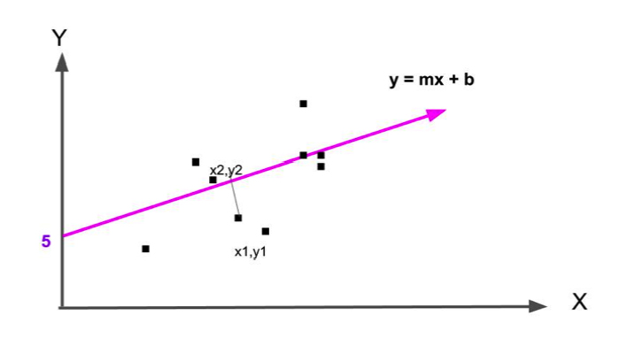
The classic way to solve this problem is to find the line
y = mx + b
that most nearly splits this data right down the middle as shown in the graph below. To do this we find the line whose average distance from the data points is smallest.
The easiest way to find that line in Apache Spark is to use:
org.apache.spark.mllib.regression.LinearRegressionMode.
But a more sophisticated approach is to use:
org.apache.spark.mllib.regression.LinearRegressionWithSGD
where means Stochastic Gradient Descent. For reasons beyond the scope of this document, suffice it to say that SGD is better suited to certain analytics problems than others. Which algorithm is best suited is based on lots of factors – like which makes the best estimates, the efficiency of the algorithm, the tend to overtrain an algorithm (which leads to deductions skewed by prejudicial assumptions), its sensitivity to outliers (meaning it messes up the estimate when there are data points far away from the others), etc.
The only way to know which model to use is to find the model with the lowest error, meaning the model that yields the smallest difference between the predicted values and observed values. This is what data scientists do – they try several models.
(This tutorial is part of our Apache Spark Guide. Use the right-hand menu to navigate.)
How to code linear regression with Apache Spark and Scala
Download this data:
https://raw.githubusercontent.com/cloudera/spark/master/mllib/data/ridge-data/lpsa.data
It does not matter what this data is. We are not interested in the column headings or even knowing what this data means. We just want to show how to do linear regression and need some data that will correlate. Much data does not correlate at all, meaning linear regression or any kind of statistics will not fit it. For example gas prices and gas sales are hardly correlated as people buy gas regardless of the price, because they need it.
First, we show the whole code then we will go through it line by line.
import org.apache.spark.mllib.linalg.Vectors
import org.apache.spark.mllib.regression.LabeledPoint
import org.apache.spark.mllib.feature.Normalizer
import org.apache.spark.mllib.regression.LinearRegressionWithSGD
val data = sc.textFile("/home/walker/lpsa.dat")
val parsedData = data.map { line =>
val x : Array[String] = line.replace(“,”, ” “).split(” “)
val y = x.map{ (a => a.toDouble)}
val d = y.size – 1
val c = Vectors.dense(y(0),y(d))
LabeledPoint(y(0), c)
}.cache()
val numIterations = 100
val stepSize = 0.00000001
val model = LinearRegressionWithSGD.train(parsedData, numIterations, stepSize)
val valuesAndPreds = parsedData.map { point =>
val prediction = model.predict(point.features)
(point.label, prediction)
}
valuesAndPreds.foreach((result) => println(s”predicted label: ${result._1}, actual label: ${result._2}”))
val MSE = valuesAndPreds.map{ case(v, p) => math.pow((v – p), 2) }.mean()
println(“training Mean Squared Error = ” + MSE)
Create LabelPoint object
First we use the textFile method to read the text file lpsa.dat, whose first lines is shown below. In this data set, y is value that we want to calculate (the dependant variable). It is the first field. The other fields are the independent variables. So instead of having just y = mx + b, where x is an input variable. Here we have many x’s.
-0.4307829,-1.63735562648104 -2.00621178480549 -1.86242597251066 -1.02470580167082 -0.522940888712441 -0.863171185425945 -1.04215728919298 -0.864466507337306
That creates data as an RDD[String].
val data = sc.textFile("/home/walker/lpsa.dat")
A string is an iterable object so we loop over it twice to split it by spaces. We do it twice because you can see in the data that the first two elements are separated by a comma so we have to get rid of that first.
val parsedData = data.map { line =>
val x : Array[String] = line.replace(",", " ").split(" ")
We then convert all these strings to Doubles, as machine learning requires numbers and this particular algorithm requires a Vector of Doubles.
val y = x.map{ (a => a.toDouble)}
The LabeledPoint is an object required by the linear regression algorithm. It is in this format
(labels, features)
Where features is a Vector. Here we use a dense vector which is a type that does not handle blank values, of which we have none.
val parsedData = data.map { line =>
val x : Array[String] = line.replace(",", " ").split(" ")
val y = x.map{ (a => a.toDouble)}
val d = y.size - 1
val c = Vectors.dense(y(0),y(d))
LabeledPoint(y(0), c)
}.cache()
Note that we use the word cache because Spark is a distributed system. To calculate this we need to retrieve data from each node. Cache, like collect, gathers all the elements across the nodes.
Training with testing data
In this example, we use the training set as the testing data as well. That is OK for purposes of illustration as both should be nearly the same if they represent true samples of actual data. In real life, you train on the training data, like the lpsa.dat file. Then you make predictions on new incoming data, which is called testing data even though a better name would be live data.
There are two parameters: numIterations and stepSize, in addition to the LabeledPoint. You would have to understand the Stochastic Gradient Descent logic and math to know what those mean, which we do not explain here as it is complex. Basically it means how many times can the algorithm keep looping to adjust its estimation, meaning hone in on the point where the error goes to as close to zero as possible. That is called converging.
val numIterations = 100
val stepSize = 0.00000001
val model = LinearRegressionWithSGD.train(parsedData, numIterations, stepSize)
Test the model
Now, to see how well it works, loop through the LabelPoint and then run the predict() method over each creating a new RDD(double, double) of the label (y or the independent variable, meaning the observed end result y) and the prediction (the estimation based on the regression formula determined by the SDG algorithm).
val valuesAndPreds = parsedData.map { point =>
val prediction = model.predict(point.features)
(point.label, prediction)
}
Calculate error
An error of 0 would mean we have a perfect model. As you can see below, the model does not do a good job of predicting values until the label is high. For the whole model, the error is:
println("training Mean Squared Error = " + MSE)
training Mean Squared Error = 7.451030996001437
MSE means the difference between the average((predicted value – actual value ) ** 2 (squared)). When the predictive nearly equals the actual value then MSE is close to 0.
valuesAndPreds.foreach((result) => println(s"predicted label: ${result._1}, actual label: ${result._2}"))
predicted label: -0.4307829, actual label: -6.538896995115336E-8
...
predicted label: 1.446919, actual label: 1.7344923653317994E-7
...
predicted label: 2.6567569, actual label: 3.4906394367410936E-7
predicted label: 1.8484548, actual label: 2.592863859023973E-7
....
predicted label: 2.2975726, actual label: 3.16412860478681E-7
predicted label: 2.7180005, actual label: 3.4164515319254127E-7
predicted label: 2.7942279, actual label: 3.448229999917885E-7
predicted label: 2.8063861, actual label: 3.5506022919177794E-7
predicted label: 2.8124102, actual label: 3.64517218758205E-7
predicted label: 2.8419982, actual label: 3.508992428582512E-7
...
predicted label: 4.029806, actual label: 5.019849314865162E-7
predicted label: 4.1295508, actual label: 5.211902354094908E-7
predicted label: 4.3851468, actual label: 5.732554699437345E-7
predicted label: 4.6844434, actual label: 6.026343831319147E-7
predicted label: 5.477509, actual label: 7.208914981741786E-7
These postings are my own and do not necessarily represent BMC's position, strategies, or opinion.
See an error or have a suggestion? Please let us know by emailing blogs@bmc.com.