The importance of data analytics is steadily growing across all industries. Having proper data analytics and visualizations tools has become more important than ever. Jupyter Notebooks is one of the leading open-source tools for developing and managing data analytics.
Jupyter initially started its life as an offshoot of the iPython project in 2014, and it’s evolved into a full-fledged interactive data science platform. Managed by the non-profit Project Jupyter organization, Jupyter aims to provide the most comprehensive data science platform.
In this article, we’ll show you how to set up and configure a local Jupyter environment. You can use this tutorial as the perfect starting point for beginning data analytics work.
What is a Jupyter Notebook?
Jupyter Notebook is an open-source web application that provides an interactive computational environment. It produces documents (notebooks) that combine both inputs (code) and outputs into a single file. It offers a single document that contains:
- Visualizations
- Mathematical equations
- Statistical modeling
- Narrative text
- Any other rich media
This single document approach enables users to develop, visualize the results and add information, charts, and formulas that make work more understandable, repeatable, and shareable.
Jupyter notebooks support more than 40 programming languages, with a major focus on Python. Since it is a free and open-source tool, anyone can use it freely for their data science projects. There are two variants of the Jupyter notebook:
- Jupyter Classic Notebook, with all the capabilities mentioned above.
- JupyterLab, a new next-generation notebook interface designed to be much more extensible and modular, with support for a wide variety of workflows from data science, machine learning, and scientific computing.
Today, JupyterLab is the default notebook for any Jupyter project.
(Get started with these Python tools.)
Installing Jupyter Notebook (JupyterLab)
There are multiple ways to install and use Jupyter Notebooks, ranging from installing via conda, mamba, pip, pipenv, or even as a Docker container.
In this section, we discuss two methods of installing Jupyter Notebooks in your local environment. (Please refer to the official documentation of Jupyter Notebook for all the installation methods.) We will be using Windows as the operating system environment for setting up JupyterLab.
Install via Pipenv
Pipenv allows users to create a deterministic reproducible virtual environment with proper dependency management for Python projects. As Jupyter comes as a pip package, we can simply install it in this virtual environment.
First, let’s create a folder that acts as the virtual environment. In this example, we have a folder called “jupyter_notebook” which will be used to create the environment using Pipenv.
Simply run the following command to initiate this folder and set up the Python version to 3.8. However, we can use any supported Python version for this.
| pipenv –python 3.8 |
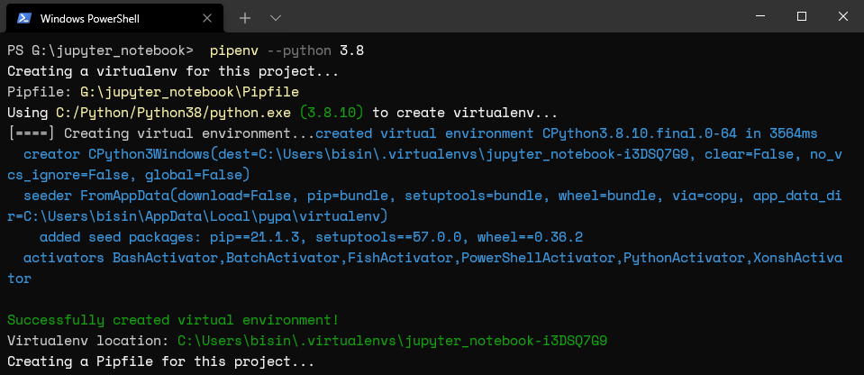
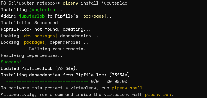
Then run the following command to install the Jupyter package via pip:
| pipenv install jupyterlab |
Finally, we can run the JupyterLab using the run command.
| pipenv run jupyter lab |
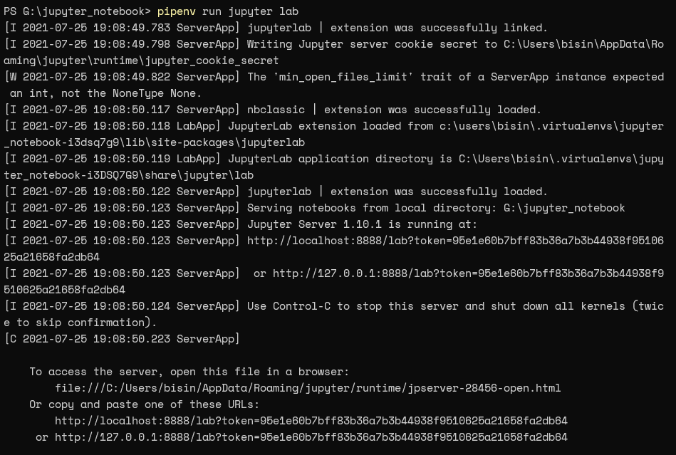
After running the JupyterLab, we will be able to access the JupyterLab installation via the provided URL (https://localhost:8888).
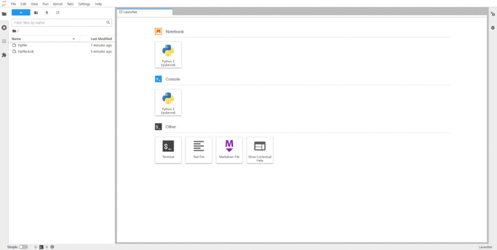
This way, the Pipenv method offers an isolated JupyterLab environment to work without conflicting with:
- Any other Python project
- Settings
- Globally installed packages
Install via Anaconda data science toolkit
Anaconda is an open-source distribution of Python and R programming languages that aims to simplify deployment and package management. It comes with its own:
- Package management system (conda)
- Virtual environment capabilities
- Software packages geared toward data science projects
The anaconda individual edition enables you to quickly set up a local data science environment by simply installing the anaconda installation package.
Now, let’s install Jupyter Notebook via Anaconda. First, navigate the Anaconda website and download the appropriate Individual Edition installation package for your operating system environment.

Then install the software in the local machine using the installer (.exe package).

After that, open the newly installed application called Anaconda Navigator once the installation is complete. It is the GUI used to install applications and packages for the conda environment. You will notice that both Jupyter Notebook and JupyterLab are available in the application section of Anaconda Navigator.
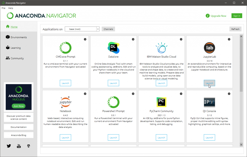
Next, select your preferred notebook type and install it. After that, click on the “Launch” button to start the Jupyter Notebook. This will open a browser window with the notebook opened.
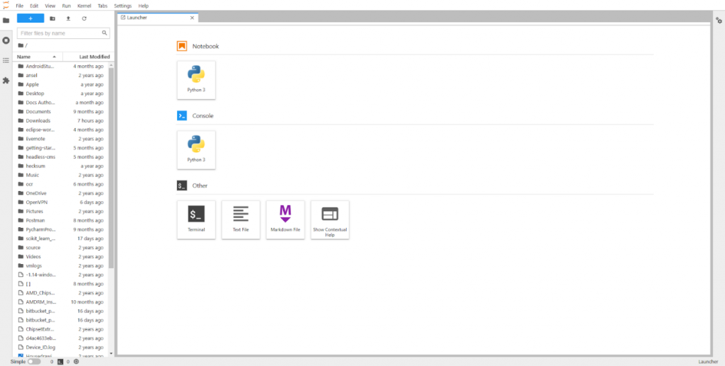
By default, Juptyper will gain access to all the files and folders within the startup location. This is the installation location for anaconda, whereas it’s the folder location of the virtual environment for Pipenv.
Creating a notebook
Since we have completed the installation process, we can now move onto creating a Notebook. Click on the notebook button on the home page of the JupyterLab web interface or navigate to File -> New -> Notebook to create a new notebook.
This will open a new untitled notebook called untitled.ipynb, where we can start coding our project.

Components of Jupyter notebook
In this section, we will cover the main components of the Jupyter notebook that are essential for interacting with the Jupyter environment.
The ipynb file
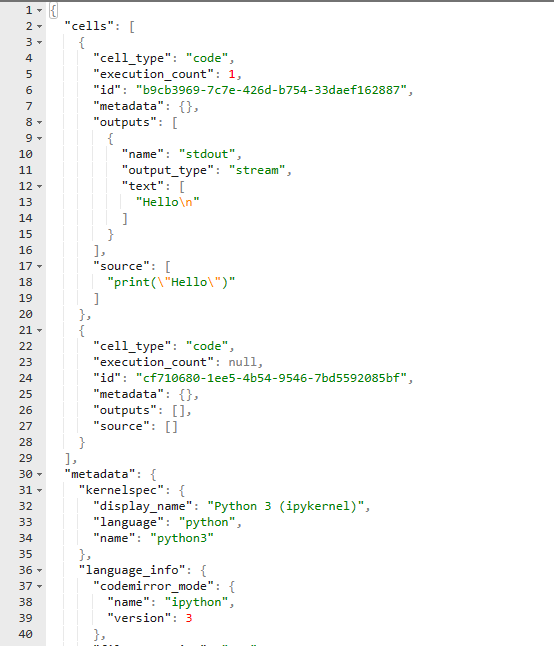
The .ipynb file is the extension used to define a single notebook. This file contains all the data of your notebook in JSON format. Moreover, it includes all the cell contents, image attachments as converted strings, and metadata related to the notebook.
Let’s create a simple notebook named test.ipynb and add a simple print statement there as shown below.
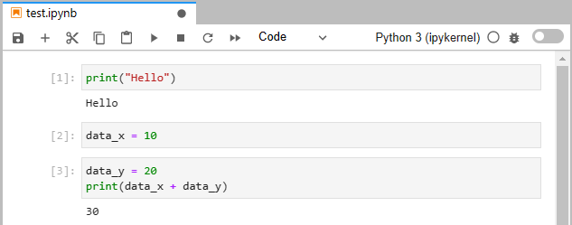
Now, if we open the test.ipynb file as a JSON file, we can see how all the information related to the notebook is stored there.
Notebook kernel
Kernel acts as the brain of the notebook. Any code within a cell will be executed in the Kernel, and the output is returned to the notebook. Kernel views the whole document (notebook) as a single entity and maintains the state between cells.
In the following example, we have defined a variable (data_x) on a cell and accessed the same variable in a separate cell for a simple addition calculation.

If we need to clear all the variables, we can simply restart the Kernel or use other options like “Restart and Clear All Outputs” or “Run All Cells” depending on the required outcome. Further, we have the interrupt option to stop the kernel if it is stuck due to a computational issue.
The kernel also dictates the programming language supported in the notebook ranging from Java, Scala, R, Lua, etc. Moreover, users can install any supported kernel and use it to create a notebook. Some kernels like the SoS kernel extend support for multiple languages in a single notebook.
Cells in a notebook
Cells are the building blocks of a notebook. Anything we do in a notebook, we do it within a specific cell block. There are two types of cells in a notebook:
- Code cell. These cells contain the code that will be executed in the kernel. When the notebook is executed, the resulting output will be shown below the code cell (outside the cell).
- Markdown cell. These cells contain the text content using Markdown. At the runtime, the result will be generated at the place of the markdown cell.
Cell types:
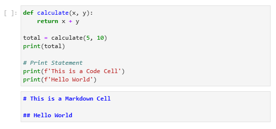
Cells at runtime:

There are two modes for all types of cells called edit and command mode:
- When we click on a cell and start editing, it will change its appearance with a blue border to indicate the edit mode.
- When we move out of the cell, it will change to a grey box to indicate the command mode.
Cell edit mode:
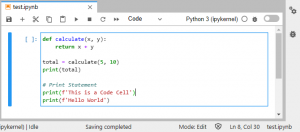
Cell command mode:

Getting started with data analytics
Now that we can install Jupyter Notebooks and understand its core components, let’s perform some data analytics and visualizations using the Notebook.
First, we will create a new notebook named “race_data.” We will use the Formula 1 World Championship (1950-2021) dataset available from Kaggle for this analysis.
The objective of this analysis is to identify the driver with the most number of wins in F1. Before getting started, make sure you have installed the required libraries for the Python environment. You can use the “pipenv install” command to install Pipenv and use conda to install anaconda.
Step 1
Import the data from the Kaggle dataset (.csv file) to Pandas data frames.
| import numpy as np import pandas as pd# Import Data results_dataframe = pd.read_csv(‘G:\data\results.csv’) circuits_dataframe = pd.read_csv(‘G:\data\circuits.csv’) drivers_dataframe = pd.read_csv(‘G:\data\drivers.csv’) races_dataframe = pd.read_csv(‘G:\data\races.csv’) constructor_dataframe = pd.read_csv(‘G:\data\constructors.csv’) |

Step 2
Verify the import by printing some data frames.
| # Prints Results Data Frame results_dataframe.head()# Prints Drivers Data Frame drivers_dataframe.head() |
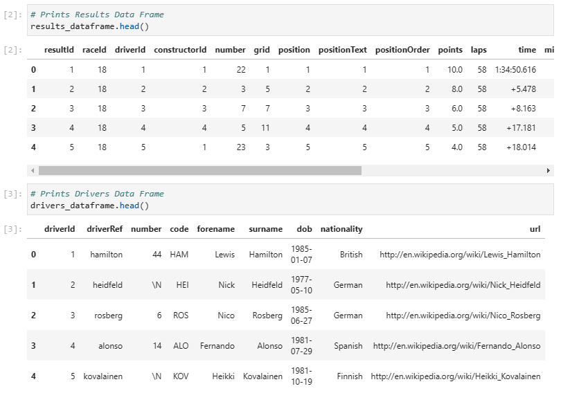
Step 3
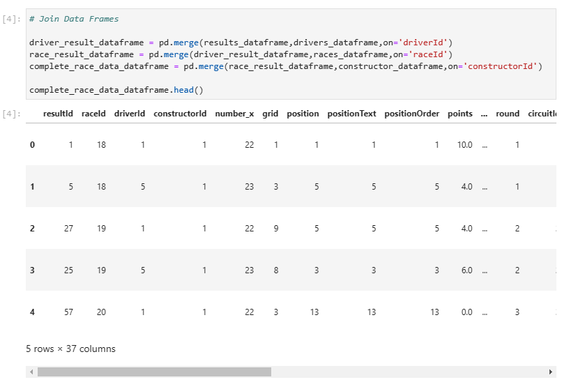
Join all the data frames to create a single primary data frame consisting of all the required data.
| # Join Data Frames driver_result_dataframe = pd.merge(results_dataframe,drivers_dataframe,on=’driverId’) complete_race_data_dataframe.head() |
Step 4
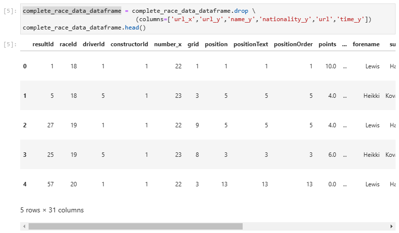
Clean the data frame. We will remove all the unnecessary columns from the data frame.
| complete_race_data_dataframe = complete_race_data_dataframe.drop (columns=[‘url_x’,’url_y’,’name_y’,’nationality_y’,’url’,’time_y’]) complete_race_data_dataframe.head() |
Step 5
Calculate the total wins for each driver. In the below code block, we:
- Filter out race data to contain only the first position finishes and create a new integer column called “position_mod.”
- Group the data by the “driverRef ” and “nationality_x” columns with the sum of the postion_mod.
- Sort the data by descending order and retrieve the first ten rows.
| # Filter & Calculate Results total_wins = complete_race_data_dataframe[(complete_race_data_dataframe[‘position’]== ‘1’)] total_wins[‘position_mod’] = total_wins[‘position’].astype(int) total_wins = total_wins.groupby([‘driverRef’,’nationality_x’])[‘position_mod’].sum().reset_index() total_wins = total_wins.sort_values(by=[‘position_mod’], ascending=False) total_wins = total_wins.head(10) |

Step 6
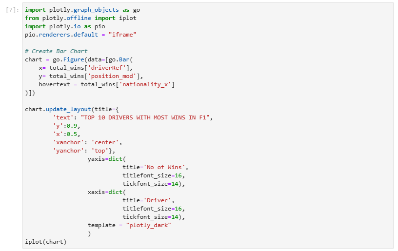
Create a bar chart using the new data set retrieved in Step 5 utilizing the plotly library.
| import plotly.graph_objects as go from plotly.offline import iplot import plotly.io as pio pio.renderers.default = “iframe”# Create Bar Chart chart = go.Figure(data=[go.Bar( x= total_wins[‘driverRef’], y= total_wins[‘position_mod’], hovertext = total_wins[‘nationality_x’] )])chart.update_layout(title={ ‘text’: “TOP 10 DRIVERS WITH MOST WINS IN F1”, ‘y’:0.9, ‘x’:0.5, ‘xanchor’: ‘center’, ‘yanchor’: ‘top’}, yaxis=dict( title=’No of Wins’, titlefont_size=16, tickfont_size=14), xaxis=dict( title=’Driver’, titlefont_size=16, tickfont_size=14), template = “plotly_dark” ) iplot(chart) |
Created chart

Begin data analytics with Jupyter
Jupyter Notebooks is the ideal place to get a head start in the data analytics field. Jupyter provides a feature-rich, robust, and user-friendly environment using multiple installation methods. Users can utilize Jupyter in any environment regardless of the platform.
Related reading
- BMC Machine Learning & Big Data
- Enabling the Citizen Data Scientists
- Data Science Certifications: An Introduction
- Data Architecture Explained: Components, Standards & Changing Architectures
- Supervised, Unsupervised & Other Machine Learning Methods
- Data Ethics for Companies
These postings are my own and do not necessarily represent BMC's position, strategies, or opinion.
See an error or have a suggestion? Please let us know by emailing blogs@bmc.com.

