
Here we show how to use Amazon AWS Machine Learning to do linear regression. In a previous post, we explored using Amazon AWS Machine Learning for Logistic Regression.
To review, linear regression is used to predict some value y given the values x1, x2, x3, …, xn. in other words it finds the coefficients b1, b2, b3, … , bn plus an offset c to yield this formula:
y = b1x1 + b2x2 + b3x3 + …. + c.
It uses the least squares error approach to find this formula. In other words, think of all these values x1, x2, … existing in some N-dimensional space. The line y is the line that minimizes the distance between the observed and predicted values for all these values. So it is the line that most nearly split right down the middle of the data observed in the training set. Since we know what that line looks like, we can take any new data, plug those into the formula, and then make a prediction.
As always models are built like this:
- Take an input set of data that you think it correlated. Such as hours of exercise and weight reduction.
- Split that data into a training set and testing set. Amazon does that splitting for you.
- Run the linear regression algorithm to find the formula for y. Amazon picks linear regression based upon the characteristics of the data. It would pick another type of regression or classification model is we picked a data set that for which that was a better fit.
- Check how accurate the model is by taking the square root of the differences between the observed and predicted values. Amazon actually uses the mean of this difference.
- Then take new data and apply the formula y to make a prediction.
Get Some Data
We will use this data of student test scores from the UCI Machine Learning repository.
I copied this data into Google Sheets here so that you can more easily read it. Plus I show the training data set and the one used for prediction.
You download this data in raw format and upload it to Amazon S3. But first, we have to delete the column headings and change the semicolon (;) separators to commas (,) as shown below. We take the first 400 rows as our model training data and the last 249 for prediction. Use vi to delete the first from the data as Amazon will not read the schema automatically (Too bad it does not).
vi student-por.csv
sed -i 's/;/,/g' student-por.csv
head -400 student-por.csv > grades400.csv
tail -249 student-por.csv > grades249.csv
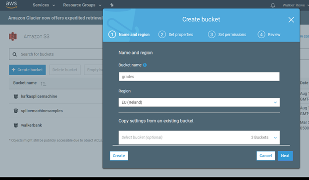
Now create a bucket in S3. I called it gradesml. Call yours some different name as it appears bucket names have to be unique across all of S3.
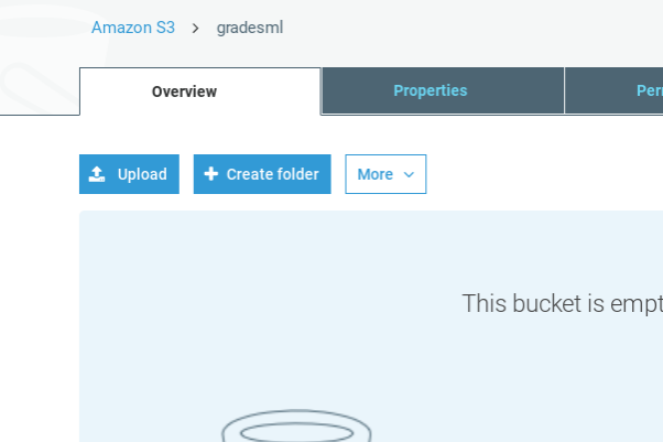
Then upload all 3 files.
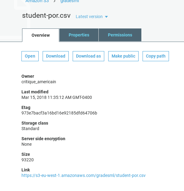
Note the https link and make sure the permissions are set to read.
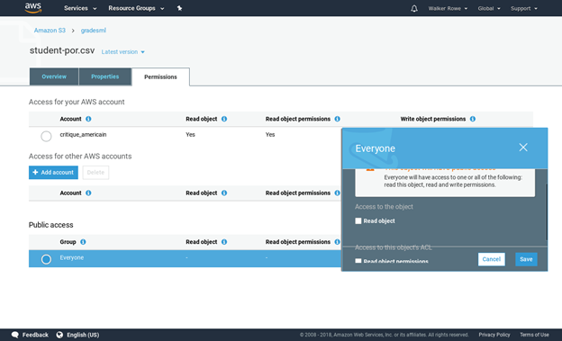
Give read permissions:
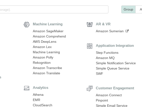
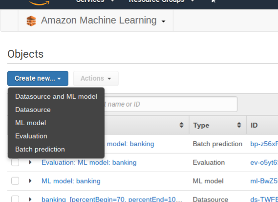
Click on Amazon Machine Learning and then Create New Data Source/ML Model. If you have not used ML before it will ask you to sign up. Creating and evaluating models is free. Amazon charges you for using them to make prediction on a per 1,000 record basis.
Click create new Datasource and ML model.
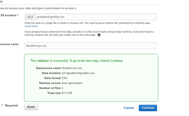
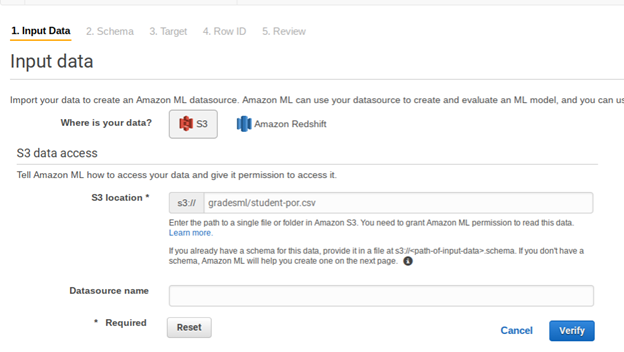
Fill in the S3 location below. Notice that you do not use the URL. Intead, put the bucket name and file name:
Click verify and Grant Permissions on the screen that pops up next.
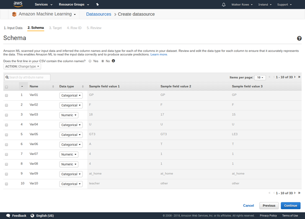
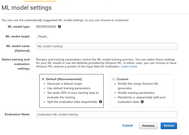
Give the data source some name then click through the screens. It fill make up field names (we actually don’t care what names it uses since we know what each column means from the original data set). It will also determine whether each value is categorical (drawn from a finite set) or just a number. What is important for you to do is to pick the target. That is the dependant value you want it to predict, i.e., y. From the input data student-por.csv pick G3, as that is the student’s final grade. These grades are from the Portuguese grammar school system and 13 is the highest value.
Below don’t use students-por.csv as the input data. Instead use grades400.csv.
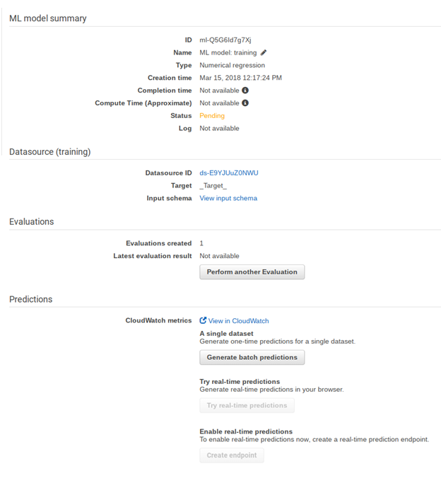
Now Amazon builds the model. This will take a few minutes.
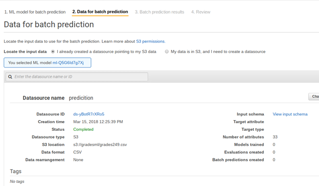
While waiting are create another data set. This is not a model so it will not ask you for a target. Use the grades249.csv file in S3, which we will use in the batch prediction step.

Now the evaluation is done. We can see which one it is from the list above as it says evaluation. Click on it. We explain what it means below.
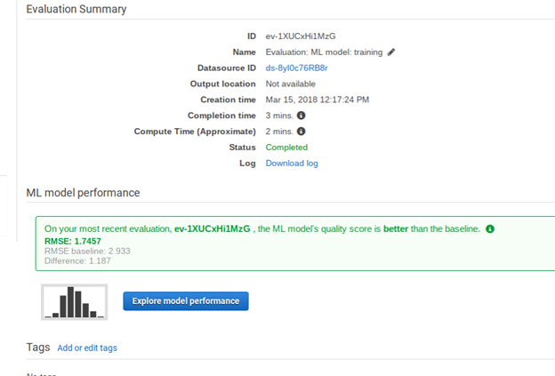
Amazon shows the RMSE. This is the square root of the sum of the squared differences of the observed and predicted values. We square and then take the square root so that all the numbers are positive, so they do not cancel each other out. Amazon also uses the mean, meaning average, by multiplying this sum by 1 / n, where n is the sample size.
If the model and the evaluations were the same, this number would be 0. So the closer to o zero we get the more accurate is our model. If the number is large, then the problem is not the algorithm, it is the data. So we could not pick another algorithm to make it much better. There is really only one algorithm used for LR, finding the least squares error. (There are more esoteric ones.) If MSE number is large then either the data is not correlated or, more like, most of the data is correlated, but some of it is not and is thus messing up our model. What we would do is drop some columns out and rebuild out model to get a more accurate model.
What value means the model is good? The model is good when the distribution of errors is a normal distribution, i.e., the bell curve.
Put another way, click Explore Model Performance.
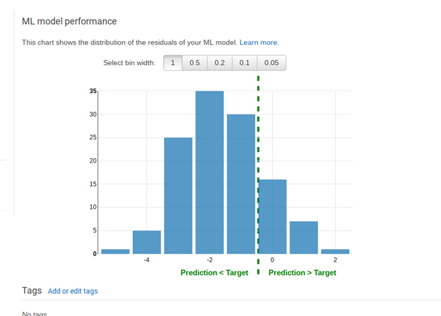
See the histogram above. Numbers to the left of the dotted line are where the predicted values were less than the observed ones. Numbers to the right are where they are higher. If this distribution were entered on the number 0 then we would have a completely random distribution. That is the idea situation where our errors are distributed randomly. But since it is shifted there is something in our data that we should leave out. For example, family size might not be correlated to grades.
Above Amazon showed the RMSE baseline. This is what the RMSE would be if we could have an input data set in which there was this perfect distribution of errors.
Also here we see the limitations of doing this kind of analysis in the cloud. If we have written our own program we could have calculated other statistics that showed exactly which column was messing up our model. Also we could try different algorithms to get rid of the bias caused by outliers, meaning numbers far from the mean that distort the final results.
Run the Prediction
Now that the model is saved, we can use it to make predictions. In other words we want to say given these student characteristics what are their likely final grades going to be.
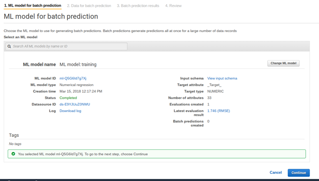
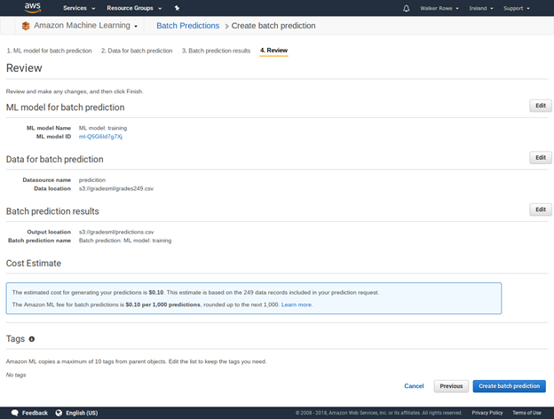
Select the prediction datasource you created above then select Generate Batch Predictions. Then click through the following screens.

Click review then create ML model.
Here we tell it where to save the results in S3. There it will save several files. The one we are interested in is the one where it calculates the score. It should tack it onto the input data to make it easier to read. But it does not. So I have pasted it into this spreadsheet for you on the sheet called prediction and added back the column headings. I also then added a column to show how the MSE mean squared error is calculated.
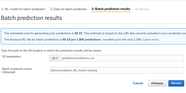

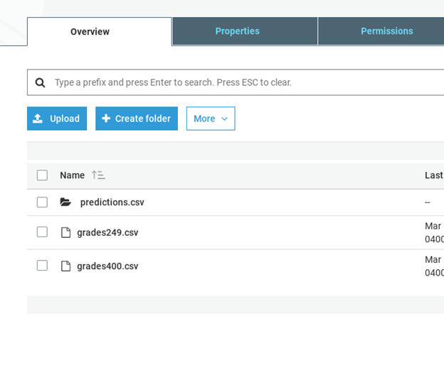
As you can see, it saves the data in S3 in a folder called predictions.csv. In this case it gave the prediction values in a file with this long name bp-ebhjggKYchO-grades249.csv.gz. You cannot view that online in S3. So download it showing the URL below and look at it with another tool. In this case I pasted the data into Google Sheets.
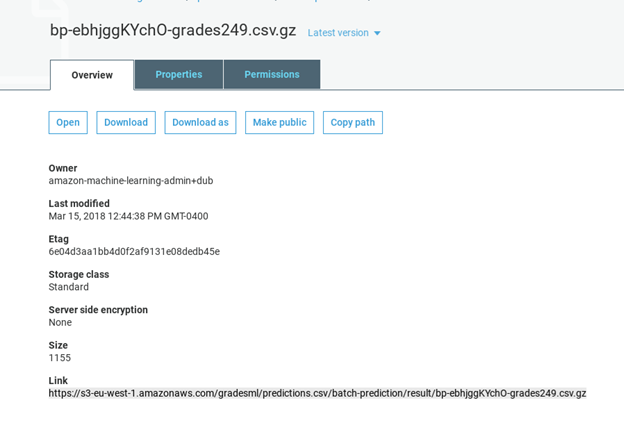
Download the data like this:
wget https://s3-eu-west-1.amazonaws.com/gradesml/predictions.csv/batch-prediction/result/bp-ebhjggKYchO-grades249.csv.gz
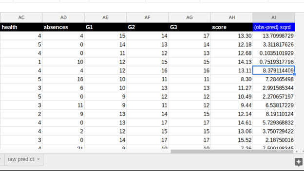
Here is that the data looks like with the prediction added to the right to make it easy to see. Column AG is the student’s actual grade. AH is the predicted value. AI is the square of the difference. And then at the bottom is MSE.
These postings are my own and do not necessarily represent BMC's position, strategies, or opinion.
See an error or have a suggestion? Please let us know by emailing blogs@bmc.com.