
Continuing with our explanations of how to measure the accuracy of an ML model, here we discuss two metrics that you can use with classification models: accuracy and receiver operating characteristic area under curve. These are some of the metrics suitable for classification problems, such a logistic regression and neural networks. There are others that we will discuss in subsequent blog posts.
For data, we use this this data set posted by an anonymous statistics professor. The Zeppelin notebook for the code shown below is stored here.
The Code
We use Pandas and scikit-learn to do the heavy lifting. We read the data into a dataframe then take two slices, x is columns 2 through 16. x is the column labeled ‘Buy’. Since this is a logistic regression problem y is equal to either 1 or 0.
import pandas as pd

url = 'https://raw.githubusercontent.com/werowe/logisticRegressionBestModel/master/KidCreative.csv'

data = pd.read_csv(url, delimiter=',')

y=data['Buy']
x = data.iloc[:,2:16]
Next we use two of the classification metrics available to us: accuracy and roc_auc. We explain those below.
First, we can comment on cross-validation, used in the algorithm below. We use model_selection.cross_val_score with cv=kfold. Basically, what this does is test predictions against observed values by looping over different divisions of the input data and taking the average of the area. This is helpful mainly with small data sets when you don’t have enough training data to split it into test, training, and validation sets.
from sklearn import model_selection
from sklearn.linear_model import LogisticRegression

for scoring in["accuracy", "roc_auc"]:
    seed = 7
    kfold = model_selection.KFold(n_splits=10, random_state=seed)
    model = LogisticRegression()
    results = model_selection.cross_val_score(model, x, y, cv=kfold, scoring=scoring)
    print("Model", scoring, " mean=", results.mean() , "stddev=", results.std())
Results in:
Model accuracy mean= 0.8886084284460052 stddev= 0.03322328503979156
Model roc_auc mean= 0.9185419071788103 stddev= 0.05710985874305497
And the individual scores:
print ("scores", results)
Model accuracy  mean= 0.8886084284460052 stddev= 0.03322328503979156
scores [0.88235294 0.83823529 0.91176471 0.89552239 0.92537313 0.91044776
 0.92537313 0.82089552 0.89552239 0.88059701]

Model roc_auc  mean= 0.9185419071788103 stddev= 0.05710985874305497
scores [0.93459119 0.92618224 0.95555556 0.94871795 0.94242424 0.89298246
 0.93874644 0.75471698 0.93993506 0.95156695]
According to Wikipedia, accuracy and precision are defined to be “In simplest terms, given a set of data points from repeated measurements of the same quantity, the set can be said to be precise if the values are close to each other, while the set can be said to be accurate if their average is close to the true value of the quantity being measured.”
Then the ROC: “A receiver operating characteristic (ROC), or simply ROC curve, is a graphical plot which illustrates the performance of a binary classifier system as its discrimination threshold is varied. It is created by plotting the fraction of true positives out of the positives (TPR = true positive rate) vs. the fraction of false positives out of the negatives (FPR = false positive rate), at various threshold settings”
In other words a threshold is set and then the ratio of false positive and false negatives is calculated.
We calculate that as shown below. We can run this calculation on the training data. In other words we feed the actual y values and the predicted ones, model.predict(x), into roc_curve().
model.fit(x, y)
predict = model.predict(x)
from sklearn.metrics import roc_curve
fpr, tpr, thresholds = roc_curve(y, predict)
print ("fpr=", fpr)
print ("tpr=", tpr)
print ("thresholds=", thresholds)
results in:
fpr= [0.         0.05839416 1.        ]
tpr= [0.    0.664 1.   ]
thresholds= [2 1 0]
We can calculate the area under the curve the receiver operating characteristic (ROC) curve:
auc = roc_auc_score(y, predict)
print (auc)
Results in:
0.8028029197080292
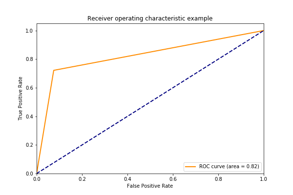
We can plot the ROC curve like this:
import matplotlib.pyplot as plt
from sklearn.metrics import roc_curve, auc

fpr = dict()
tpr = dict()
roc_auc = dict()

n_classes = 2
for i in range(n_classes):
    fpr[i], tpr[i], _ = roc_curve(predict, y)
    roc_auc[i] = auc(fpr[i], tpr[i], auc(y,predict, reorder=True))

plt.figure()
lw = 2
plt.plot(fpr[0], tpr[0], color='darkorange',lw=lw, label='ROC curve (area = %0.2f)' % roc_auc[0])
plt.plot([0, 1], [0, 1], color='navy', lw=lw, linestyle='--')
plt.xlim([0.0, 1.0])
plt.ylim([0.0, 1.05])
plt.xlabel('False Positive Rate')
plt.ylabel('True Positive Rate')
plt.title('Receiver operating characteristic example')
plt.legend(loc="lower right")
plt.show()
Results in this plot: