Bias–Variance Tradeoff in Machine Learning: Concepts & Tutorials
Every data engineer must develop an understanding of the bias and variance tradeoff in machine learning (ML).
ML is used in more applications every day. Speech and image recognition, fraud detection, chatbots, and generative AI, are now commonplace uses of this technology. The growing use of ML is bringing the intricacies of how machine learning algorithms work out of specialized labs and into the mainstream of information technology.
Machine learning models cannot be a black box. Data engineers and users of large data sets must understand how to create and evaluate various algorithms and learning requirements when building and evaluating their ML models. Bias and variance in machine learning affect the overall accuracy of any model (which can be interpreted from a confusion matrix), trust in its outputs and outcomes, and its capacity to train machines to learn.
In this article, we will discuss what bias and variance in machine learning are. We will also touch on how to deal with the bias and variance tradeoff in developing useful algorithms for your ML applications.
(New to ML? Read our ML vs AI explainer.)
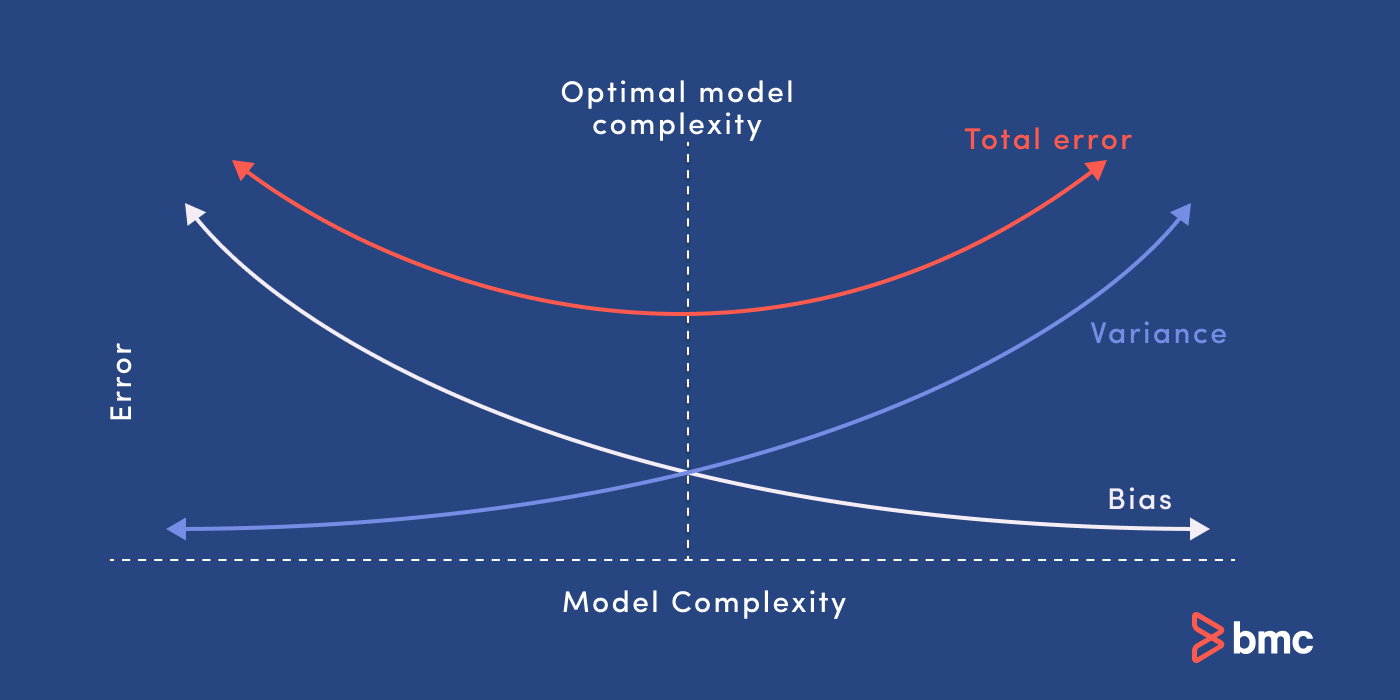
Bias and variance are two sources of error in predictive models. Getting the right balance between the bias and variance tradeoff is fundamental to effective machine learning algorithms. Here is a quick explanation of these concepts:
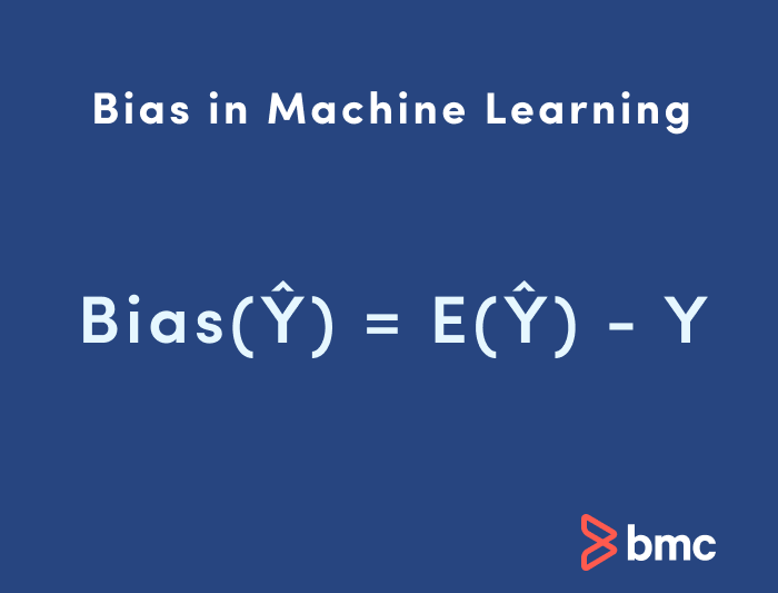 Bias in ML is sometimes called the “too simple” problem. Bias is considered a systematic error that occurs in the machine learning model itself due to incorrect assumptions in the ML process.
Technically, we can define bias as the error between average model prediction and the ground truth. Moreover, it describes how well the model matches the training data set:
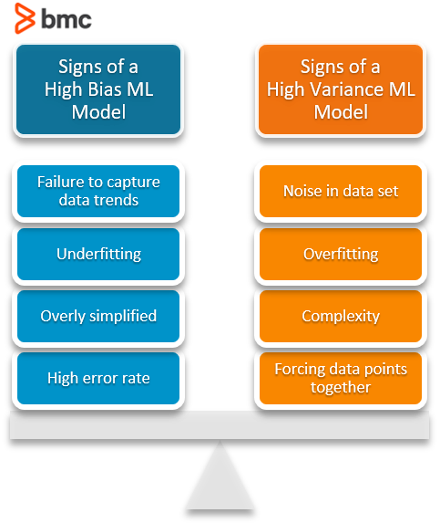
Characteristics of a high bias model include:
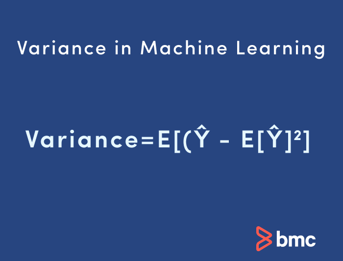 Variance in machine learning is sometimes called the “too sensitive” problem. Variance in ML refers to the changes in the model when using different portions of the training data set.
Simply stated, variance is the variability in the model prediction—how much the ML function can adjust depending on the given data set. Variance comes from highly complex models with a large number of features.
All these contribute to the flexibility of the model. For instance, a model that does not match a data set with a high bias will create an inflexible model with a low variance that results in a suboptimal machine learning model.
Characteristics of a high variance model include:
You can see from our fruit example how important it is that your model matches the data. How well your model “fits” the data directly correlates to how accurately it will perform in making identifications or predictions from a data set.
Bias and variance are inversely connected. It is impossible to have an ML model with a low bias and a low variance.
When a data engineer modifies the ML algorithm to better fit a given data set, it will lead to low bias—but it will increase variance. This way, the model will fit with the data set while increasing the chances of inaccurate predictions.
The same applies when creating a low variance model with a higher bias. While it will reduce the risk of inaccurate predictions, the model will not properly match the data set.
It’s a delicate balance between these bias and variance. Importantly, however, having a higher variance does not indicate a bad ML algorithm. Machine learning algorithms should be able to handle some variance.
We can tackle the trade-off in multiple ways…
A large data set offers more data points for the algorithm to generalize data easily. However, the major issue with increasing the trading data set is that underfitting or low bias models are not that sensitive to the training data set. Therefore, increasing data is the preferred solution when it comes to dealing with high variance and high bias models.
This table lists common algorithms and their expected behavior regarding bias and variance:
| Algorithm | Bias | Variance |
| Linear Regression | High Bias | Less Variance |
| Decision Tree | Low Bias | High Variance |
| Bagging | Low Bias | High Variance (Less than Decision Tree) |
| Random Forest | Low Bias | High Variance (Less than Decision Tree and Bagging) |
Let’s put these concepts into practice—we’ll calculate bias and variance using Python.
The simplest way to do this would be to use a library called mlxtend (machine learning extension), which is targeted for data science tasks. This library offers a function called bias_variance_decomp that we can use to calculate bias and variance.
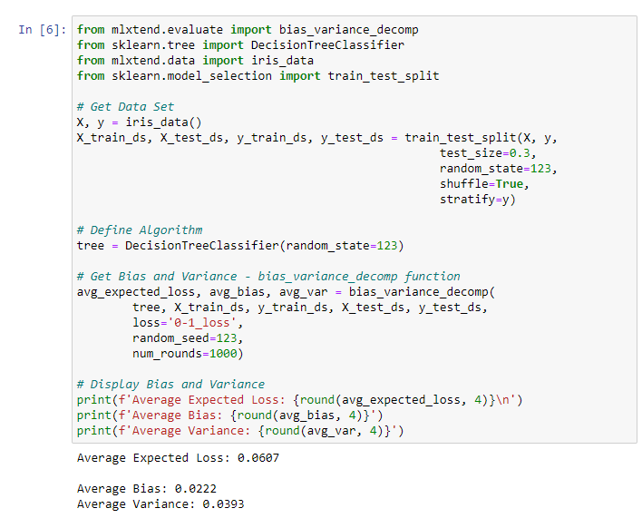
We will be using the Iris data data set included in mlxtend as the base data set and carry out the bias_variance_decomp using two algorithms: Decision Tree and Bagging.
from mlxtend.evaluate import bias_variance_decomp
from sklearn.tree import DecisionTreeClassifier
from mlxtend.data import iris_data
from sklearn.model_selection import train_test_split

# Get Data Set
X, y = iris_data()
X_train_ds, X_test_ds, y_train_ds, y_test_ds = train_test_split(X, y,
                                                    test_size=0.3,
                                                    random_state=123,
                                                    shuffle=True,
                                                    stratify=y)

# Define Algorithm
tree = DecisionTreeClassifier(random_state=123)

# Get Bias and Variance - bias_variance_decomp function
avg_expected_loss, avg_bias, avg_var = bias_variance_decomp(
        tree, X_train_ds, y_train_ds, X_test_ds, y_test_ds,
        loss='0-1_loss',
        random_seed=123,
        num_rounds=1000)

# Display Bias and Variance
print(f'Average Expected Loss: {round(avg_expected_loss, 4)}n')
print(f'Average Bias: {round(avg_bias, 4)}')
print(f'Average Variance: {round(avg_var, 4)}')
Result:
from mlxtend.evaluate import bias_variance_decomp
from sklearn.tree import DecisionTreeClassifier
from mlxtend.data import iris_data
from sklearn.model_selection import train_test_split
from sklearn.ensemble import BaggingClassifier

# Get Data Set
X, y = iris_data()
X_train_ds, X_test_ds, y_train_ds, y_test_ds = train_test_split(X, y,
                                                    test_size=0.3,
                                                    random_state=123,
                                                    shuffle=True,
                                                    stratify=y)

# Define Algorithm
tree = DecisionTreeClassifier(random_state=123)
bag = BaggingClassifier(base_estimator=tree,
                        n_estimators=100,
                        random_state=123)

# Get Bias and Variance - bias_variance_decomp function
avg_expected_loss, avg_bias, avg_var = bias_variance_decomp(
        bag, X_train_ds, y_train_ds, X_test_ds, y_test_ds,
        loss='0-1_loss',
        random_seed=123,
        num_rounds=1000)

# Display Bias and Variance
print(f'Average Expected Loss: {round(avg_expected_loss, 4)}n')
print(f'Average Bias: {round(avg_bias, 4)}')
print(f'Average Variance: {round(avg_var, 4)}')
Result:
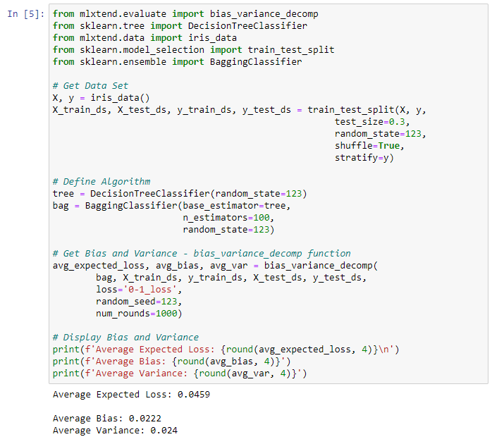 Each of the above functions will run 1,000 rounds (num_rounds=1000) before calculating the average bias and variance values. We can reduce the variance without affecting bias, using a bagging classifier. The higher the algorithm complexity, the lower the variance.
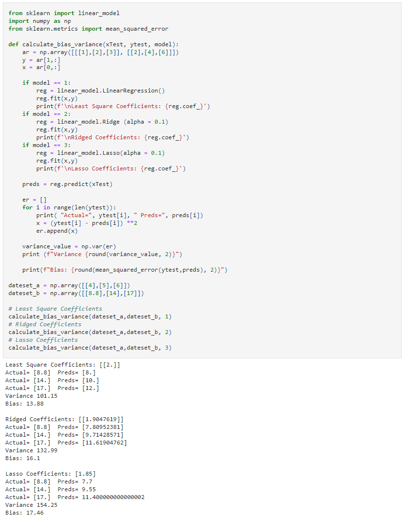
In the following example, we will look at three different linear regression models: least-squares, ridge, and lasso, using sklearn library. Since they are all linear regression algorithms, their main difference will be the coefficient value.
We can see those different algorithms lead to different outcomes in the ML process (bias and variance).
from sklearn import linear_model
import numpy as np
from sklearn.metrics import mean_squared_error

def calculate_bias_variance(xTest, ytest, model):
    ar = np.array(,,], ,,]])
    y = ar
    x = ar

    if model == 1:
        reg = linear_model.LinearRegression()
        reg.fit(x,y)
        print(f'nLeast Square Coefficients: {reg.coef_}')
    if model == 2:
        reg = linear_model.Ridge (alpha = 0.1)
        reg.fit(x,y)
        print(f'nRidged Coefficients: {reg.coef_}')
    if model == 3:
        reg = linear_model.Lasso(alpha = 0.1)
        reg.fit(x,y)
        print(f'nLasso Coefficients: {reg.coef_}')

    preds = reg.predict(xTest)

    er = []
    for i in range(len(ytest)):
        print( "Actual=", ytest, " Preds=", preds)
        x = (ytest - preds) **2
        er.append(x)

    variance_value = np.var(er)
    print (f"Variance {round(variance_value, 2)}")

    print(f"Bias: {round(mean_squared_error(ytest,preds), 2)}")

dateset_a = np.array(,,])
dateset_b = np.array(,,])

# Least Square Coefficients
calculate_bias_variance(dateset_a,dateset_b, 1)
# Ridged Coefficients
calculate_bias_variance(dateset_a,dateset_b, 2)
# Lasso Coefficients
calculate_bias_variance(dateset_a,dateset_b, 3)
Result:
Bias and variance are two key components that you must consider when developing any good, accurate machine learning model.
Users need to consider both these factors when creating an ML model. Generally, your goal is to keep bias as low as possible while introducing acceptable levels of variances. This can be done either by increasing the complexity or increasing the training data set.
In this balanced way, you can create an acceptable machine learning model.