
Amazon SageMaker is a managed machine learning service (MLaaS). SageMaker lets you quickly build and train machine learning models and deploy them directly into a hosted environment. In this blog post, we’ll cover how to get started and run SageMaker with examples.
One thing you will find with most of the examples written by Amazon for SageMaker is they are too complicated. Most are geared toward working with handwriting analysis etc. So here we make a new example, based upon something simpler: a spreadsheet with just 50 rows and 6 columns.
Still, SageMaker is far more complicated than Amazon Machine Learning, which we wrote about here and here. This is because SageMaker is not a plug-n-play SaaS product. You do not simply upload data and then run an algorithm and wait for the results.
Instead SageMaker is a hosted Jupyter Notebook (aka iPython) product. Plus they have taken parts of Google TensorFlow and scikit-learn ML frameworks and written the SageMaker API on top of that. This greatly simplifies TensorFlow programming.
SageMaker provides a cloud where you can run training jobs, large or small. As we show below, it automatically spins up Docker containers and runs your training model across as many CPUs, GPUs, and memory that you need. So it lets you write and run ML models without having to provision EC2 virtual machines yourself to do that. It does the container orchestration for you.
What you Need to Know
In order to follow this code example, you need to understand Jupyter Notebooks and Python.
Jupyter is like a web page Python interpreter. It lets you write code and execute it in place. And it lets you draw tables and graphs. With it you can write programs, hide the code, and then let other users see the results.
Pricing
SageMaker is not free. Amazon charges you by the second. In writing this paper Amazon billed me $19.45. If I had used it within the first two months of signing up with Amazon it would have been free.
SageMaker Notebook
To get started, navigate to the Amazon AWS Console and then SageMaker from the menu below.
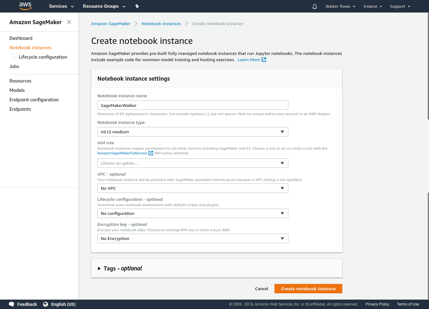
Then create a Notebook Instance. It will look like this:
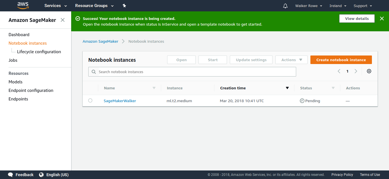
Then you wait while it creates a Notebook. (The instance can have more than 1 notebook.)
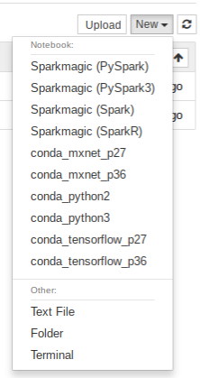
Create a notebook. Use the Conda_Python3 Jupyter Kernel.
 |
KMeans Clustering
In this example, we do KMeans clustering. That takes an unlabeled dataset and groups them into clusters. In this example, we take crime data from the 50 American states and group those. So we can then show which states have the worst crime. (We did this previously using Apache Spark here.) We will focus on getting the code working and not interpreting the results.
Download the data from here. And change these columns headings:
,crime$cluster,Murder,Assault,UrbanPop,Rape
To something easier to read:
State,crimeCluster,Murder,Assault,UrbanPop,Rape
Alabama,4,13.2,236,58,21.2
Alaska,4,10,263,48,44.5
Arizona,
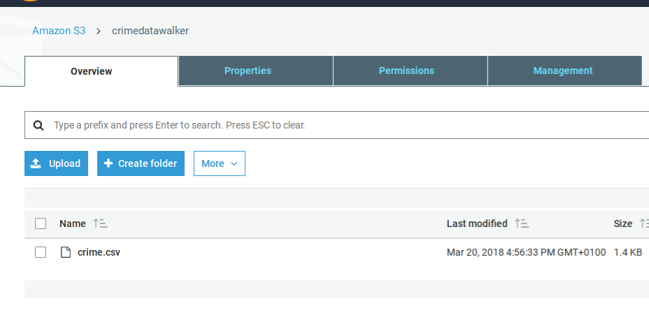
Amazon S3
You need to upload the data to S3. Set the permissions so that you can read it from SageMaker. In this example, I stored the data in the bucket crimedatawalker. Amazon S3 may then supply a URL.
Amazon will store your model and output data in S3. You need to create an S3 bucket whose name begins with sagemaker for that.
Basic Approach
Our basic approach will be to read the comma-delimited data into a Pandas dataframe. Then we create a numpy array and pass that to the SageMaker KMeans algorithm. If you have worked with TensorFlow, you will understand that SageMaker is far easier than using that directly.
We also use SageMaker APIs to create the training model and execute the jobs on the Amazon cloud.
The Code
You can download the full code from here. It is a SageMaker notebook.
Now we look at parts of the code.
The %sc line below is called Jupyter Magic. The %sc means run a shell command. In this case we download the data from S3 so that the file crime.csv can be read by the program.
%sc
!wget 'https://s3-eu-west-1.amazonaws.com/crimedatawalker/crime_data.csv'
Next we read the csv file crime_data.csv into a Pandas Dataframe. We convert the state values to numbers since numpy arrays must contain only numeric values. We will also make a cross reference so that later we can print the state name in text given the numeric code.
As the end we convert the dataframe to a numpy array of type float32. The KMeans algorithm expects the float32 format (They call it dtype).
import pandas as pd
import numpy as np
import matplotlib.pyplot as plt
crime = pd.read_csv('crime_data.csv', header=0)
print(crime.head())
This subroutine converts every letter of the state name to its ASCII integer representation then adds them together.
def stateToNumber(s):
l = 0
for x in s:
l = l + int(hex(ord(x)),16)
return l
Here we change the State column in the dataframe to its numeric representation.
xref = pd.DataFrame(crime['State'])
crime['State']=crime['State'].apply(lambda x: stateToNumber(x))
crime.head()
Now we convert the dataframe to a Numpy array:
crimeArray = crime.as_matrix().astype(np.float32)
Here we give SageMaker the name of the S3 bucket where we will keep the output. The code below that is standard for any of the algorithms. It sets up a machine learning task.
Note that we used machine size ml.c4.8xlarge. Anyone familiar with Amazon virtual machine subscription fees will be alarmed as a machine of that size costs a lot to use. But Amazon will not let you use the tiny or small templates.
from sagemaker import KMeans
from sagemaker import get_execution_role
role = get_execution_role()
print(role)
bucket = "sagemakerwalkerml"
data_location = "sagemakerwalkerml"
data_location = 's3://{}/kmeans_highlevel_example/data'.format(bucket)
output_location = 's3://{}/kmeans_example/output'.format(bucket)
print('training data will be uploaded to: {}'.format(data_location))
print('training artifacts will be uploaded to: {}'.format(output_location))
kmeans = KMeans(role=role,
train_instance_count=1,
train_instance_type='ml.c4.8xlarge',
output_path=output_location,
k=10,
data_location=data_location)
Now we run this code and the Jupyter Notebook cells above it. Then we can stop there since we will now have to wait for Amazon to complete the batch job it creates for us.
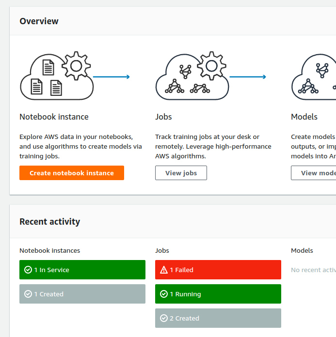
Amazon creates a job in SageMaker which we can then see in the Amazon SageMaker dashboard (See below.). Also you will see that the cell in the notebook will have an asterisk (*) next to it, meaning it is busy. Just wait until the asterisk goes away. Then Amazon will update the display and you can move to the next step.
Here is what it looks like when it is done.
arn:aws:iam::782976337272:role/service-role/AmazonSageMaker-ExecutionRole-20180320T064166
training data will be uploaded to: s3://sagemakerwalkerml/kmeans_highlevel_example/data
training artifacts will be uploaded to: s3://sagemakerwalkerml/kmeans_example/output
Next we drop the State name (which has already been turned into a number) from the numpy array. Because the name by itself does not mean anything so we do not want to feed it into the Kmeans algorithm.
slice=crimeArray[:,1:5]
Below the magic %%time tells Jupyter that this step will take some time so wait before moving forward. kmeans.fit() means run the model using the Numpy array kmeans.record_set(numpy Array).
%%time
kmeans.fit(kmeans.record_set(slice))
Amazon will respond saying it has kicked off this job. Then we wait 10 minutes or so for it to complete.
INFO:sagemaker:Creating training-job with name: kmeans-2018-03-27-08-32-53-716
The SageMaker Dashboard
Now go look at the SageMaker Dashboard and you can see the status of jobs you have kicked off. They can take some minutes to run.
When the job is done it writes this information to the SageMaker notebook. You can can see it created a Docker container to run this algorithm.
Docker entrypoint called with argument(s): train
[03/27/2018 14:11:37 INFO 139623664772928] Reading default configuration from /opt/amazon/lib/python2.7/site-packages/algorithm/default-input.json: {u'_num_gpus': u'auto', u'local_lloyd_num_trials': u'auto', u'_log_level': u'info', u'_kvstore': u'auto', u'local_lloyd_init_method': u'kmeans++', u'force_dense': u'true', u'epochs': u'1', u'init_method': u'random', u'local_lloyd_tol': u'0.0001', u'local_lloyd_max_iter': u'300',
u'_disable_wait_to_read': u'false', u'extra_center_factor': u'auto', u'eval_metrics': u'["msd"]', u'_num_kv_servers': u'1', u'mini_batch_size': u'5000', u'half_life_time_size': u'0', u'_num_slices': u'1'}
…
[03/27/2018 14:11:38 INFO 139623664772928] Test data was not provided.
#metrics {"Metrics": {"totaltime": {"count": 1, "max": 323.91810417175293, "sum": 323.91810417175293, "min": 323.91810417175293}, "setuptime": {"count": 1, "max": 14.310121536254883, "sum": 14.310121536254883, "min": 14.310121536254883}}, "EndTime": 1522159898.226135, "Dimensions": {"Host": "algo-1", "Operation": "training", "Algorithm": "AWS/KMeansWebscale"}, "StartTime": 1522159898.224455}
===== Job Complete =====
CPU times: user 484 ms, sys: 40 ms, total: 524 ms
Wall time: 7min 38s
Deploy the Model to Amazon SageMaker Hosting Services
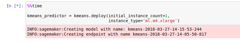
Now we deploy the model to SageMaker using kmeans.deploy().
%%time
kmeans_predictor = kmeans.deploy(initial_instance_count=1,
instance_type='ml.m4.xlarge')
Amazon responds:
INFO:sagemaker:Creating model with name: kmeans-2018-03-27-09-07-32-599
INFO:sagemaker:Creating endpoint with name kmeans-2018-03-27-08-49-03-990
And we can see that the Notebook is busy because there is an asterisk next to the item in Jupyter.
The next step is to use the model and see how well it works. We will feed 1 record into it before we run the whole test data set against it. Here we use the same crime_data.csv data for the train and test data set. The normal approach is to split those into 70%/30%. Then you get brand new data and plug that in when you make predictions.
First take all the rows but drop the first column.
slice=crimeArray[:,1:5]
slice.shape
slice
Now grab just one row for our initial test.
s=slice[1:2]
Now run the predict() method. Take the results and turn it into a dictionary. Then print the results.
%%time
result = kmeans_predictor.predict(s)
clusters = [r.label['closest_cluster'].float32_tensor.values[0] for r in result]
i = 0
for r in result:
out = {
"State" : crime['State'].iloc[i],
"StateCode" : xref['State'].iloc[i],
"closest_cluster" :  r.label['closest_cluster'].float32_tensor.values[0],
"crimeCluster" : crime['crimeCluster'].iloc[i],
"Murder" :  crime['Murder'].iloc[i],
"Assault" : crime['Assault'].iloc[i],
"UrbanPop" : crime['UrbanPop'].iloc[i],
"Rape" :  crime['Rape'].iloc[i]
}
print(out)
i = i + 1
Here are the results. For that first record, it has placed it in cluster 6. It also calculated the mean squared distance, which we did not print out.
{'State': 671, 'StateCode': 'Alabama', 'closest_cluster': 7.0, 'crimeCluster': 4, 'Murder': 13.199999999999999, 'Assault': 236, 'UrbanPop': 58, 'Rape': 21.199999999999999}
And now all 50 states.
%%time
result = kmeans_predictor.predict(slice)
clusters = [r.label['closest_cluster'].float32_tensor.values[0] for r in result]
i = 0
for r in result:
out = {
"State" : crime['State'].iloc[i],
"StateCode" : xref['State'].iloc[i],
"closest_cluster" :  r.label['closest_cluster'].float32_tensor.values[0],
"crimeCluster" : crime['crimeCluster'].iloc[i],
"Murder" :  crime['Murder'].iloc[i],
"Assault" : crime['Assault'].iloc[i],
"UrbanPop" : crime['UrbanPop'].iloc[i],
"Rape" :  crime['Rape'].iloc[i]
}
print(out)
i = i + 1
{'State': 671, 'StateCode': 'Alabama', 'closest_cluster': 1.0, 'crimeCluster': 4, 'Murder': 13.199999999999999, 'Assault': 236, 'UrbanPop': 58, 'Rape': 21.199999999999999}
{'State': 589, 'StateCode': 'Alaska', 'closest_cluster': 7.0, 'crimeCluster': 4, 'Murder': 10.0, 'Assault': 263, 'UrbanPop': 48, 'Rape': 44.5}
{'State': 724, 'StateCode': 'Arizona', 'closest_cluster': 3.0, 'crimeCluster': 4, 'Murder': 8.0999999999999996, 'Assault': 294, 'UrbanPop': 80, 'Rape': 31.0}
{'State': 820, 'StateCode': 'Arkansas', 'closest_cluster': 6.0, 'crimeCluster': 3, 'Murder': 8.8000000000000007, 'Assault': 190, 'UrbanPop': 50, 'Rape': 19.5}
{'State': 1016, 'StateCode': 'California', 'closest_cluster': 3.0, 'crimeCluster': 4, 'Murder': 9.0, 'Assault': 276, 'UrbanPop': 91, 'Rape': 40.600000000000001}
{'State': 819, 'StateCode': 'Colorado', 'closest_cluster': 6.0, 'crimeCluster': 3, 'Murder': 7.9000000000000004, 'Assault': 204, 'UrbanPop': 78, 'Rape': 38.700000000000003}
As an exercise you could run this again and drop the crimeCluster column. The data we have already includes clusters that someone else calculated. So we should get rid of that.
Note also that you cannot rerun the steps where it creates the model unless you change the data in some way. Because it will say the model already exists. But you can run any of the other cells over and over as it persists the data. For example you could experiment with adding graphs or changing the output to a dataframe to make it easier to read.
Additional Resources